Rebecca Ansorge
Elena Bollati
Ben Coppin
Sara Eisler
Luke Kelly-Granger
Group 10
June 26-July 9, 2011
Alex Griffths
Lexi Mackee
William Passfield
Rosalyn Putland
Jordan Thomas
Phillip Turner

|
|
Rebecca Ansorge Elena Bollati Ben Coppin Sara Eisler Luke Kelly-Granger |
Group 10 June 26-July 9, 2011 |
Alex Griffths Lexi Mackee William Passfield Rosalyn Putland Jordan Thomas Phillip Turner |
|
|
|
|
|
|
|
|
|
|
|
|
THE FAL ESTUARY
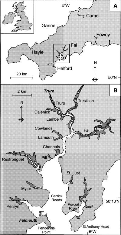
The Fal Estuary is situated on the South coast of Cornwall in the Southwest of the United Kingdom (Figure 1), it is a ria system (drowned river valley), which was developed in response to Holocene sea-level rise. The estuary extends 18 km inland from its mouth to the northern tidal limit at Tresillian and has a total shoreline length of 127 km. It can be divided into two regions: the inner tidal tributaries and the outer tidal basin, termed Carrick Roads. (Pirrie et al. 2003). Carrick Roads is a deep meandering channel reaching 34m depth at its maximum and holds 80% of the main water body of the estuary, making it an important natural harbour (Pirrie et al, Cambourne School of Mines.).
The estuary is macrotidal with a maximum spring tide of 5·3 m at Falmouth, but mesotidal at Truro with a spring tide of 3·5 m. The estuary covers 24.82 km2 with 17.36 km2 covered by the subtidal area, 6.53 km2 of intertidal mudflats and 0.93 km2 of saltmarsh (Stapleton & Pethick, 1996).
SPECIAL AREA OF CONSERVATION (SAC)
The Fal and Helford have been selected as a SAC due to the variety of habitats causing a diverse range of marine and coastal communities, such as; rocky shores, kelp forests, mearl (at St. Mawes bank) and eelgrass beds, saltmarshes and intertidal mudflats.
ACTIVITIES Within the Fal Estuary many anthropogenic activities occur that may result in significant changes to the results, especially in terms of the nutrient levels, therefore the Fal, despite its SAC status, has been labelled as one of the most polluted estuaries in the area.
Mining has taken place in the area since the Bronze age (2500-600BC), however has become much more extensive since the industrial revolution which used methods that did not necessarily protect the estuary from contamination. (Pirrie et al, Cambourne School of Mines) A notable source of pollution was after the closure of the Wheal Jane mine in January 1992, when the withdrawal of dewatering pumps lead to the extensive flooding of the estuary with 50 million tonnes of acid water carrying metal ions. (Bowen et al, 1998)
Another cause of pollution is the leeching of tributyl tin (TBT) from ships hulls that enter Falmouth Harbour continuously throughout the year, causing imposex in Nucella spp. along with suggested effects in other species.
|
Figure 1: Image of the Fal Estuary with respect to the
United Kingdom and Cornwall UK.
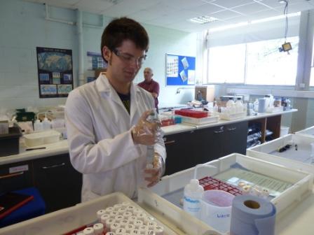
Figure 3: Group member using pipette for phosphorus
analysis
|
|
|
|
|
|
|
|
|
|
|
|
Laboratory Methods |
||||||||||||||
MEASUREMENT OF CHLOROPHYLL IN MARINE
PHYTOPLANKTON: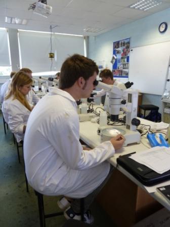 Counting Marine Phytoplankton: A 1ml subsample of the Lugol's Iodine preserved phytoplankton culture is placed in a Sedgewick-Rafter (SR) Counting Chamber and covered with a haemocytometer slide. Under 10 or 20 x magnification all the phytoplankton species in five transects of 20 squares were noted down and their abundance counted. Each square of the SR chamber represents 1µm, therefore the values recorded need to be multiplied by 20 to obtain the number of cells per ml (Purdie, 2011). Note: For chains of phytoplankton cells, the individual cells need to be recorded. Counting Marine Zooplankton: In 5ml subsamples, 10ml of the preserved zooplankton culture was analysed within a Bogorov chamber. For each sample the abundance of groups of zooplankton were recorded on a provided record sheet, using an ID guide as an aid. The groups included Copepoda, examples of jelly fish larvae (Cnidaria: Hydrozoa), as well as Decapoda, Cirripedia, Polychaeta and gastropod larvae. Following this, the numbers counted in each 10ml subsample were multiplied to provide a value for zooplankton abundance per metre cubed (Purdie, 2011).
Figure 2: Member of group 10 counting
zooplankton under a microscope
TIME TABLE June & July, 2011
Calibrations All data from CTD and YSI Probes were calibrated using standard data unless stated otherwise.
|
|
|
|
|
|
|
|
|
|
|
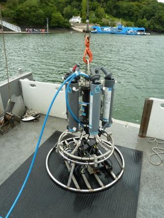
| CTD Rosette
|
Acoustic Doppler
Current Profiler
|
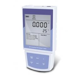
T/S Probe
|
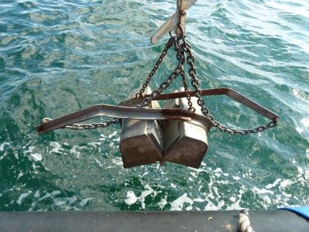
| Van Veen Grab
|
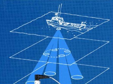
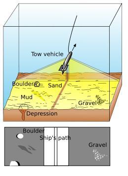
Geoacoustic Side
Scanner
|
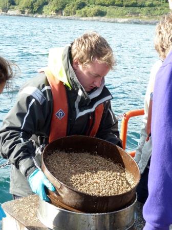
Sieve Stack
|
|
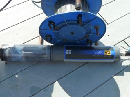
YSI 6600 Multiprobe
|
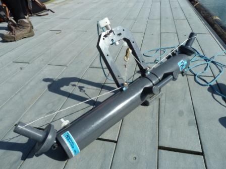
Transmissometer
|
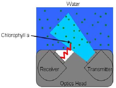
Fluorometer
|
|
Niskin Bottles
|
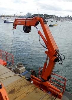
Winch
|
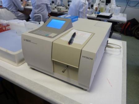
Spectrophotometer A spectrophotometer is a device that can be used to calculate a range of chemical concentrations in a solution by passing a light at a set wavelength through a cuvette containing a sometimes coloured solution. A photometer, in the device, measures how much light is absorbed by the solution. Unknown samples need to be compared to predetermined standards to calculate the concentration.
|
|
Video Sled
|
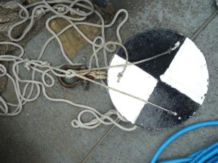
Secchi Disk
|
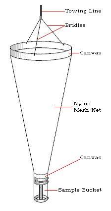
Plankton Net
|
|
|
|
|
|
|
|
|
|
|
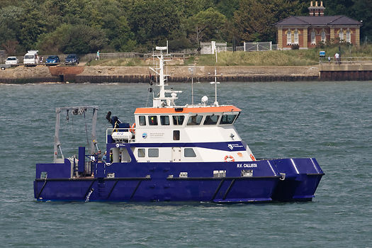
| R.V Callista
A twin hulled research vessel owned by the University of Southampton and
first dispatched in August 2005. With a passenger capacity of 30, large
working deck and onboard wet and dry lab facilities to analyse samples
the Callista is an ideal vessel for research off the South Coast.
Figure 4: Image of the R.V Callista |
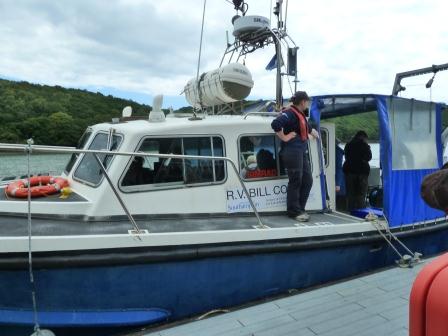
Bill Conway A Lochin 38 research vessel owned by the University of Southampton and built by Lochin Marine Ltd in 1991; which is licensed by MCA (Workboat Certificate category 2), enabling the vessel to operate up to 60 miles from security. With a passenger capacity of 12 and a limitation of single day sampling trips, the Bill Conway is ideal for smaller scale research projects.
Figure 5: Image of the Bill Conway during estuary survey in the Fal Estuary |
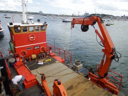
Grey Bear
Figure 6: Image of the Grey Bear docked at the Prince of Whales pier before the geophysics survey |
|
|
|
|
|
|
|
|
|
|
| Introduction | |||||||||||||||||||||
|
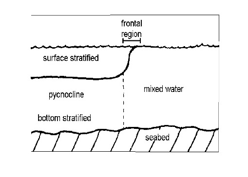
Figure 7: Image showing a shelf sea front between mixed water and
stratified water
|
|||||||||||||||||||||
| Results | |||||||||||||||||||||
|
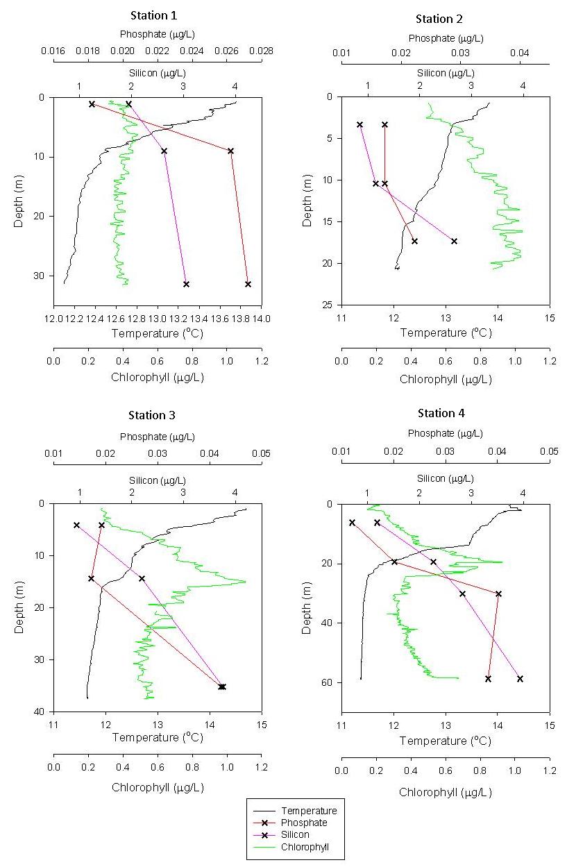
CTD DATA The CTD measures temperature, salinity, fluorescence, light intensity and turbidity within the vertical water profile (Figure 8). The calibrated fluorescence data show the chlorophyll concentration. Temperature: At station 1 the surface water temperature of 13.5°C decreases gradually down to 12.1°C at 30m. A similar trend is observed at station 2 where a relatively linear decrease in temperature within the upper 20m occurs between approximately the same temperatures as at station 1. The beginning of a very weak thermocline is seen at station 3 at 15m depth (from 12.3-11.9, and clear temperature stratification is observed at station 4 at around 20m, where the temperature decreases rapidly by 2°C from 13.5°C to 11.5°C. Both station 3 and 4 show higher surface temperatures and lower deep water temperatures than at stations 1 and 2. Fluorometer calibrated (chlorophyll): The chlorophyll concentration at station 1 remains relatively constant with depth, at station 2 the chlorophyll increases with depth, the highest concentration being between 10 and 20 meters. The chlorophyll concentration at station 3 shows a peak of 1µg/L at 15m depth. A similar chlorophyll peak of a concentration of 1µg/L is also observed at station 4 around 20m depth. Light intensity: Between stations 1 and 4 the depth of the 1% light penetration calculated from the CTD data increases from 20-21m at station 1 and 2 down to 29m at station 4. The values calculated from the CTD data do not correlate well with those calculated form the secchi depth, especially at stations 3 and 4 showed in Table O1.
Salinity: The surface salinity between the stations increases moving away from the shore (from station 1 to station 4). The salinity at each station increases gradually with depth and then remains constant after a certain value. At station 1 salinity increases to 10m and then remains constant at around 35.27PSU. At station 2 and 3 salinity increases to approximately 35.3PSU at 20m and at station 4 it increases to 35.34 at about 30m. Turbidity: The turbidity increases with depth at each of the stations. Density (calculated from the CTD data):
At stations 1, 3 and 4 the water
density increases logarithmically with depth, they show a rapid increase
in density in the surface waters which becomes a gradual increase at
depth. The graph at station 2 shows approximately a linear increase of
density with depth. At station 3 and 4 the point at with the increase
in density lessens is approximately at the base of the thermocline (15
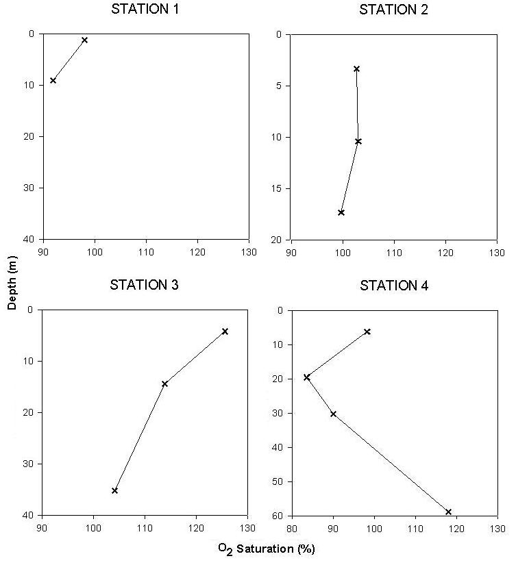
and 25m respectively). Oxygen: At station 1 there are insufficient data available to analyse the oxygen profile. Within the first 20m of station 2 there is little difference in the oxygen saturation which remains approximately 100%, in comparison, station 3 shows a high surface oxygen saturation of approximately 125% which decreases down to 105% at 35m. The oxygen saturation at station 4 shows a very different distribution with an oxygen minimum layer of about 85% observed at 20m (Figure 9). Phosphate: Comparing the phosphate concentration (Figure8) of the four stations a development of different situations can be observed. The phosphate concentration at station 1 is low in the surface waters with a weak increase down to a concentration of 0.026µg/L at 10m, which remains relatively constant in deeper water. At station 2 the first 10m also have a low phosphate concentration but this only increases slightly with depth from 0.017µg/L to 0.022µg/L at 17m. A lower phosphate concentration is seen within the upper 15m of station 3 with a steep increase to a maximum of 0.04µg/L at 35m depth. A stratification of phosphate concentration is observed at station 4; low concentrations exist in the surface 20m of the water column. The concentrations increase at approximately 30m and remain at a higher value of about 0.04µM in deeper waters. Silicon: The silicon concentration in the water column (Figure 8) at station 1 decreases weakly from 2 to 3µg/L over the water column. At station 2 a low concentration of 1µg/L exists within the upper 10m of the water column, the concentration then increases by 2.7µg/L down to 15m. At station 3 and 4 a linear increase of the silicon concentration from approximately 1 to 4µg/L is seen over the depth of the profiles. But while at station 3 a high concentration of 4µM is reached at 35m the same value is not reached until 60m at station 4 and by 35m at station 4 the silicon concentration is only 3µg/L. This shown the general trend of the silicon concentration is a decrease in the upper water column between the stations moving away from the shore.
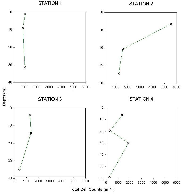
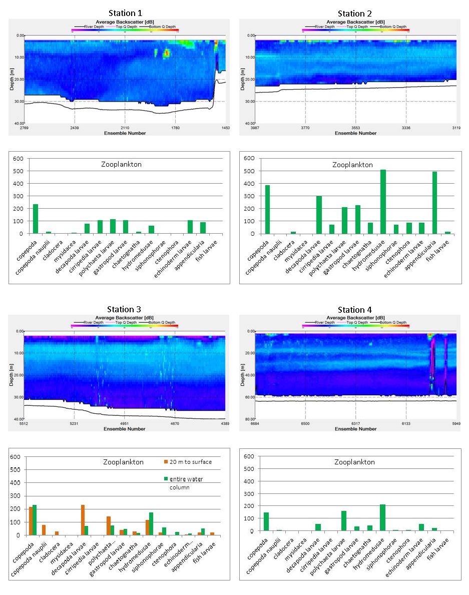
PLANKTON Phytoplankton: The number of phytoplankton individuals (Figure 10) analysed by cell counts at station 1 shows little difference within the top 30m with all values being about 1000 cells ml-1. Comparatively, at station 2 the surface phytoplankton number is very large, between 5000-6000 cells ml-1 at 5m, at 10m and below the number of cells decreases to 1000-2000 cells ml-1. Within the upper 15m of station 3 1000-2000 cells ml-1 were counted a decrease is observed to 35-40m. The data for station 4 shows a minimum in phytoplankton numbers at 20m depth. Either side of this at both 5m and 30m depth the cell numbers were between 1000-2000 cells ml-1. At 60m water depth very few phytoplankton organisms were recorded. Zooplankton and ADCP backscatter: The ADCP backscatter data are compared to the zooplankton individual counts and identification, in theory the higher the backscatter in the ADCP the higher the zooplankton number (Figure 11).
At station 1 the most abundant
zooplankton group is copepoda of which 270 individuals m-3
were recorded. Larvae of several different organisms were also recorded
at approximately 100 individuals m-3.A very high abundance
and species diversity of zooplankton is observed at station 2 where
hydromedusae and appendicularia dominate with abundances of 500
individuals m-3. Copepoda are also found in abundance (400
individuals m-3), as are decapoda larvae (300 individuals m-3).
In contrast the ADCP backscatter at this station is not high relative to
other stations. At station 3 the zooplankton numbers vary between upper
20 meters and whole water column, copepoda and decapod larvae are most
abundant within the first 20m, in the whole water column copepods and
hydromedusae dominate. At station 3 the ADCP backscatter is highest
compared to all other stations, however the counted zooplankton numbers
were highest at station 2. At station 4 two bands of high backscatter
are seen, one within the thermocline at 20m and the other one below at
30m. Zooplankton counts at this station are quite low and correlate well
with the relatively weak backscatter bands. The dominant groups are
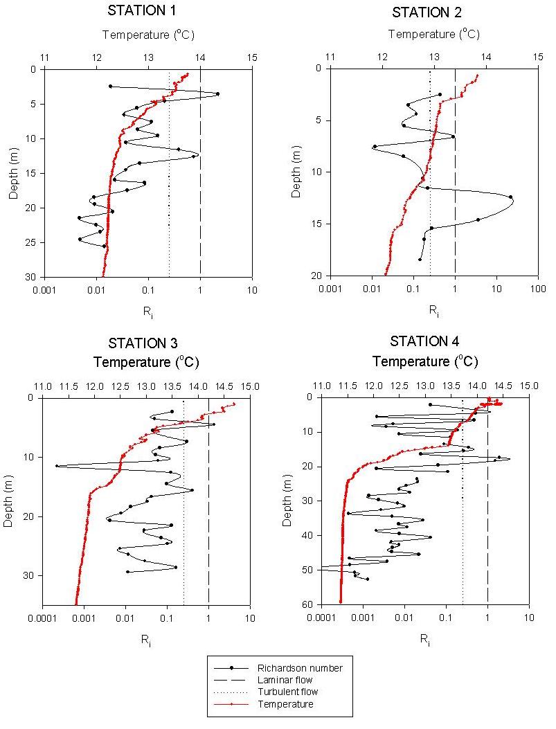
hydromedusae, polychaeta larvae and copepoda. RICHARDSON NUMBER The Richardson number (Ri) is a dimensionless number that expresses the ratio of potential energy to kinetic energy in the water column. It is an indication of turbulence. For turbulence to be maintained, the rate of kinetic energy input must exceed the potential energy demand. Ri is given by the following equation:
Where g is gravity (9.81 ms-2), r is the density, and U is the mean flow. Typically when Ri < 1, turbulence can be maintained, when Ri > 1 turbulence will either die out or be absent, and if there is no turbulent flow, the condition for it to become turbulent is when Ri < 0.25.
At station 1 the Richardson
number shows a mainly turbulent water flow except of one single data
point at 3.5m depth which is laminar. The diagram of station 2 shows a
laminar flow between 12 and 14m and a turbulent flow at most of the
depth. A turbulent flow dominates station 3 with a single data point of
laminar flow at 4.5m. Station 4 shows a laminar flow at around 18m which
is in the thermocline. Everywhere else in the water column a turbulent
or intermediate flow can be observed. The deeper layer below the
thermocline is more turbulent. POTENTIAL ENERGY ANOMALY The Potential Energy Anomaly (f) is a measurement of the amount of energy needed to mix the water column. Therefore it is also an indication of how stratified the water column is. When f > 0 the water column is stratified and when f = 0 the water column is completely vertically mixed. The potential energy anomaly is given by the following equation:
where h is the depth of the water column and r(z)
is the density at point z and
We calculated the potential energy anomaly at each station (Table O1) using the density profile data to estimate the average density of each stratification layer within the water column. From this we could determine the potential energy of the water column with the following equation:
where hc is the height of the centre of gravity and dz is the thickness of the layer of water.
The values obtained for the potential energy anomaly at each station indicates that each station had stratified water columns. As the distance away from shore increases with, as does the potential energy anomaly as to be seen in Figure 12. This indicates that the water is more stratified in the open waters as opposed to at the mouth of the estuary.
|
Click Images to Enlarge
Figure 8: Depth profiles for each of the four stations showing temperature, chlorophyll (from CTD), phosphate
and nitrate concentration (from discrete samples)
Figure 9: dissolved oxygen depth profiles for each of the four stations, obtained by titration of discrete samples.
Figure 10: depth profiles for total phytoplankton cell counts at each station.
Figure 11: ADCP backscatter profiles for each station lined up with bar charts of zooplankton counts from plankton net samples.
Figure 12: Richardson number vs depth for each station, compared with CTD temperature plots. Vertical control lines show turbulent and laminar flow thresholds.
|
||||||||||||||||||||
| Discussion | |||||||||||||||||||||
|
Analysing the calibrated data of the fluorometer from the CTD, which gives an indication of the chlorophyll concentration, the vertical profile at station 1 and 2 was seen to be relatively invariable with depth. Phytoplankton need light and nutrients to carry out primary production by photosynthesis. As chlorophyll was found relatively evenly distributed throughout the whole water column at station 1 and 2 it is likely that the organisms are being mixed into deeper water layers where light intensity is insufficient for photosynthetic processes. The temperature profiles at these stations show a decrease with depth but no clear stratification, also indicating that the whole water column is well-mixed (Sharples and Simpson, 2009). The nutrient concentrations also support this idea because nutrients are available in the entire water column, although at station 2 the nutrient concentration is lower at surface. The chlorophyll concentrations at stations 3 and 4 both peak within the thermocline. The temperature drop of 0.5°C within the slight thermocline at station 3 is very small but suggests the presence of a front nearby. A well-developed stratification with a clear thermocline occurs at station 4 and probably indicates the presence of a front. This is also supported by the density data at station 4 which shows a more stratified profile than station 1 or 2, and the Richardson numbers which show laminar flow within the thermocline (indicating stratification) and turbulent areas above and below it. Consequently the nutrient concentrations in the surface mixed layer are very low and higher below the thermocline where nutrient exchange by mixing activities can occur. The silicon in the surface waters is depleted as it is used by diatoms to build their frustules (Martin-Jézéquel et al., 2003). The phytoplankton is therefore found within the thermocline where both nutrients and light are available. At station 4 the oxygen minimum layer at 20m within the thermocline indicates high respiration rates by heterotrophic organisms feeding directly and indirectly on the high number of phytoplankton. The 1% light depth calculated from the CTD data does not correlate well with the depths calculated form the Secchi disc. This can be explained by the inaccuracies of the measurement method of the Secchi depth which can be influenced by cloud cover and boat shadow. Settling out of suspended material input from the estuary causes the 1% light depth to increase with each station moving away from the shore. The increase of the salinity with each station can be explained by increasing distance from the fresh water input of the estuary. Moving away from the estuary the fresh water is mixed into the seawater as the profile at station 4 shows while at station 1 the water is less mixed and a layer of less saline water exists at the surface. Comparing the phytoplankton data to the fluorometer data of the CTD should show good correlation. At station 1 the two measurements do correlate well and both show little change with depth. However the large increase in cell counts at the surface of station 2 is not observed in the CTD data. At station 3 and 4 the fluorometer data show maximum values at the thermocline which should also be shown in the cell counts. At station 3 the phytoplankton numbers do not increase around the thermocline and at station 4 the cell counts actually decrease. Therefore the phytoplankton cell counts are inaccurate and cannot be analysed.
Zooplankton found in the samples are mainly phytoplanktivores, therefore
their abundance should correlate with chlorophyll concentration. The
strength of the ADCP backscatter can also be used to determine the
amount of zooplankton in the water column. A high zooplankton abundance
observed at station 2 is not reflected in the backscatter and does not
correlate with the chlorophyll data. The backscatter intensity at
station 3 and 4 is relatively high around the thermocline which is to be
expected because of high chlorophyll. The backscatter at station 4 shows
an interesting picture of two bands, probably caused by zooplankton
feeding strategies. Some species are feeding within the thermocline and
some are feeding below on the rain of organic matter (e.g. faecal
pellets and dead phytoplankton). The backscatter at station 3 and 4 do
not correlate well with the zooplankton counts, suggesting the counts
are inaccurate. Errors encountered during the offshore sampling work include problems with the CTD data. As it was the first time the CTD had been used on this field course, there were a number of unrealistic data points, especially for the chlorophyll and light attenuation. At station 4, while the CTD was stationary at depth, the reading increased and then on the ascent the readings were much higher. The light sensor also behaved strangely with huge peaks on both the down cast and up cast, possibly caused by the light levels being so low that the machine malfunctioned.
During the vertical plankton trawl, readings on the flow meter appeared inaccurate. Therefore, the flow had to be calculated from diameter and mesh size. At station 3, for an unknown reason, the plankton net trawl returned purely clear water; indicating very little plankton. With this, the sample was discarded and another trawl carried out. A further issue with the plankton net was it did not close with the aid of a messenger. Due to this, instead of taking samples between certain depths, the samples were of the entire water column.
During transit, the stopper of bottle 82 came out resulting in possible contamination by the water used to keep it cool. In addition to this, the phosphate samples were not filtered before being stored, this meant that the phytoplankton was not removed and some of the phosphate may have been utilised whilst being stored.
During the laboratory work there were a few possible errors. The phosphate reagents appeared to have a contaminant floating in the bottles whilst measuring cylinders were used to measure the reagents volumes, which are less accurate than pipettes.
There were no silicon standards to work the concentration of the samples from on the day of analysis. Some standards were received several days later, however, these would not take account of small scale variations in the spectrometer.
During the dissolved oxygen analysis there were bubbles present in bottles 64, 82 and 83 bubbles, which would have affected readings.
During the chlorophyll analysis there were some differences between repeats of the same station at the same depth. In this case, the highest value was assumed to be correct as the fluorometer only measures chlorophyll, which would not give a high reading unless chlorophyll is present. A further potential error in plankton biomass estimates is within the phytoplankton and zooplankton cell counts; which, with each team member analysing separate bottles could make the counts relatively subjective as each person may see things differently and misidentify the species. |
|||||||||||||||||||||
|
Conclusion |
|||||||||||||||||||||
|
The aim of the offshore survey was to find and characterize the frontal system between the mixed water of the estuary and the stratified conditions further offshore. The front was identified at approximately station 3 where very slight stratification is found and mixing processes still occur. Furthermore the offshore stratification is clear but not as strong as it was in the previous 2 years probably caused by this years’ colder weather (weatheronline.co.uk). The phytoplankton and zooplankton distribution and abundance differes between the mixed waters, the frontal system and the stratified habitat due to water movement and nutrient and light availability. Within the mixed area nutrients and phytoplankton are relatively evenly distributed throughout the water column and no real thermocline exists. At the frontal region different conditions are seen above and below the weak thermocline in which the majority of phytoplankton and zooplankton live, however mixing processes still occur. In the stratified water at station 4 the two water layers (surface and deep water) are separated by the thermocline which is also where a high chlorophyll concentration is found. The zooplankton are feeding both within and below the thermocline. |
|||||||||||||||||||||
|
|
|
|
|
|
|
|
|
|
| Introduction | |||||||||||||||||||||||||||||||||
|
Falmouth Bay is an area of coastal water found to the
south of Falmouth town in Cornwall UK. The bay is an area
which has populations of maerl and macroalgae which ma
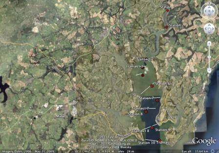
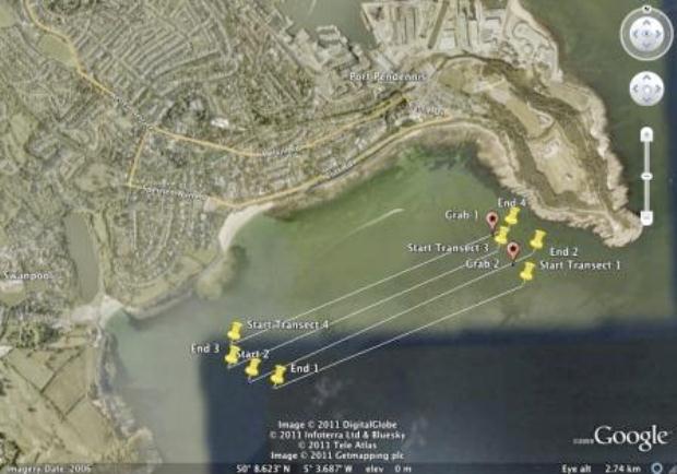
Figure 13: Google earth image showing tracts followed
during the geophysics survey
As a result of the frequent dumping of disposed sediment in this area, the benthic community in this region is often changing. This can be seen through video observations of the sea floor.
AIMS: |
|||||||||||||||||||||||||||||||||
| Methods | |||||||||||||||||||||||||||||||||
|
|
|||||||||||||||||||||||||||||||||
|
GENERAL INFORMATION: Start: 13:00 GMT
|
TIDE DATA:
|
||||||||||||||||||||||||||||||||
| Results | |||||||||||||||||||||||||||||||||
|
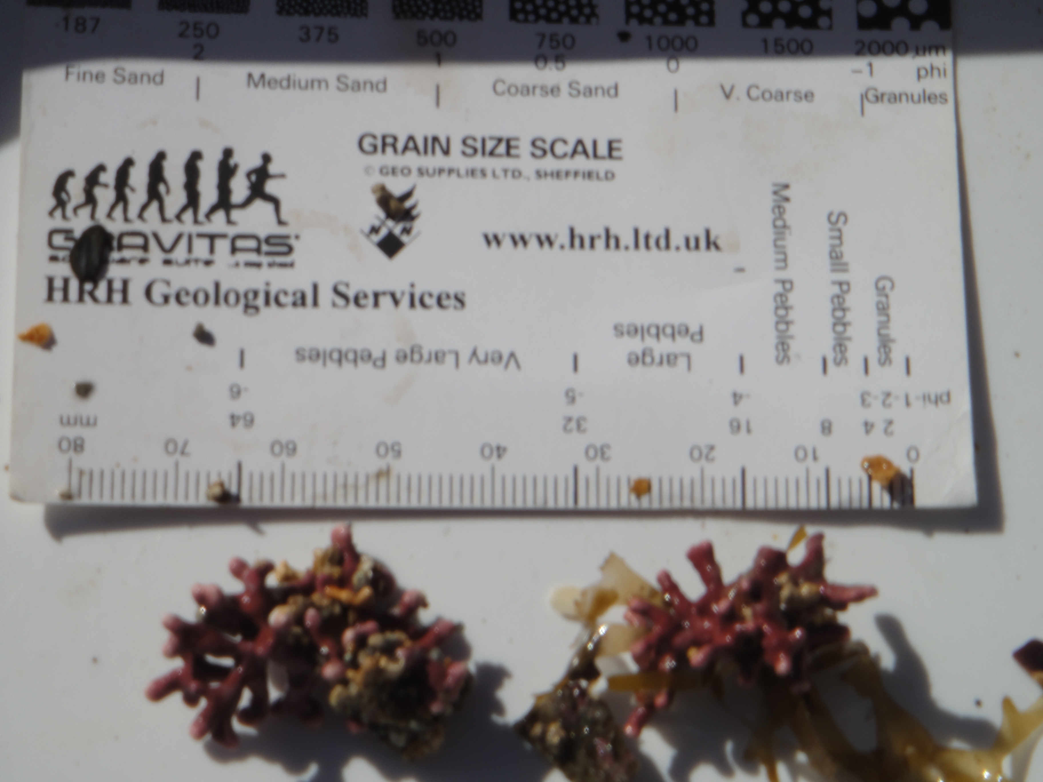
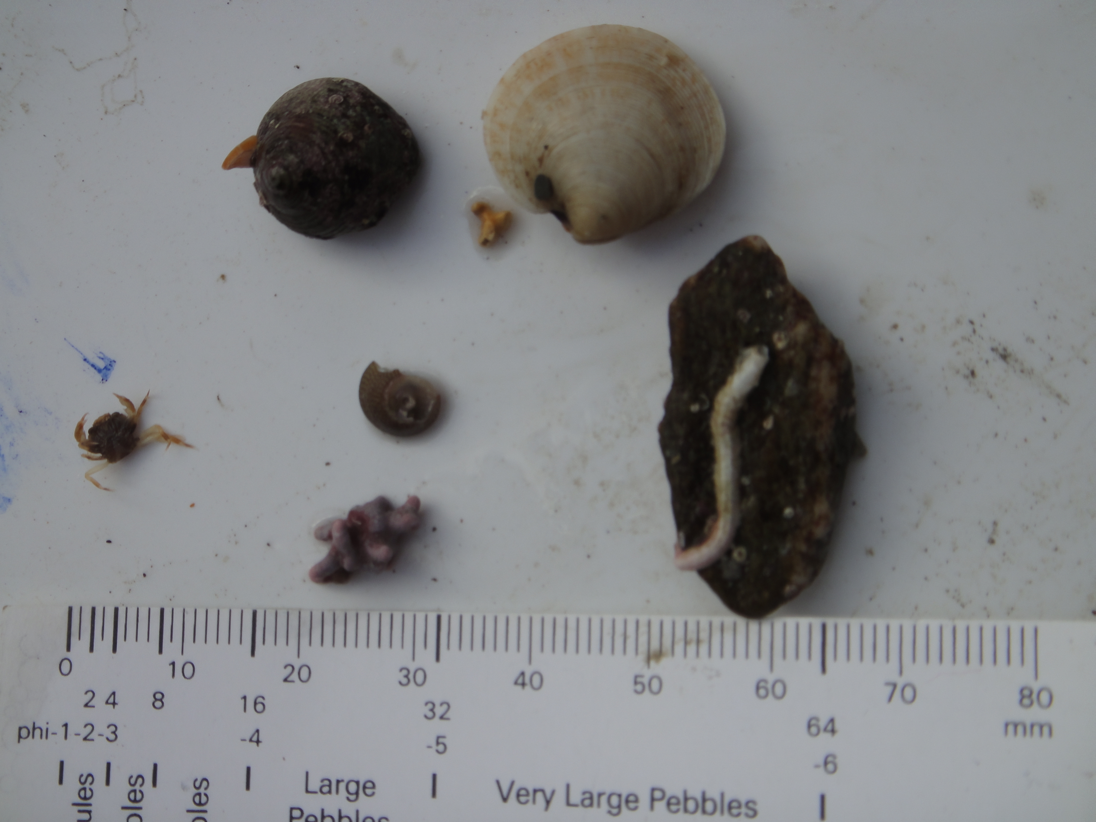
GRAB ONE: Latitude 50⁰08.625 Longitude 005⁰03.094 Eastings 182117.9780 Northings 31521.0362 Time in water (GMT) 16:01:47 DESCRIPTION: Grab had a rock caught in it when brought up but a decent sized sample was still picked up. The sample was poorly sorted and very coarse with a mixture of gravel and larger rocks, some with encrusting algae. Some shell remains and fragments of maerl were also found. BIOTA: Pea crab (Pinnotheridae spp.) ~2mm in size Gastropods Keelworm (Pomatoceros triqueter) on large rocks Chiton (Mollusca:Polyplacophora) Click Images to Enlarge
Figure 14: Pea crab (Pinnotheres pisum), grey topshell (Gibbula cineraria), venus bivalve (family: Veneroidea), alive fragment of maerl, keelworm on pebble (Pomatoceros triqueter)
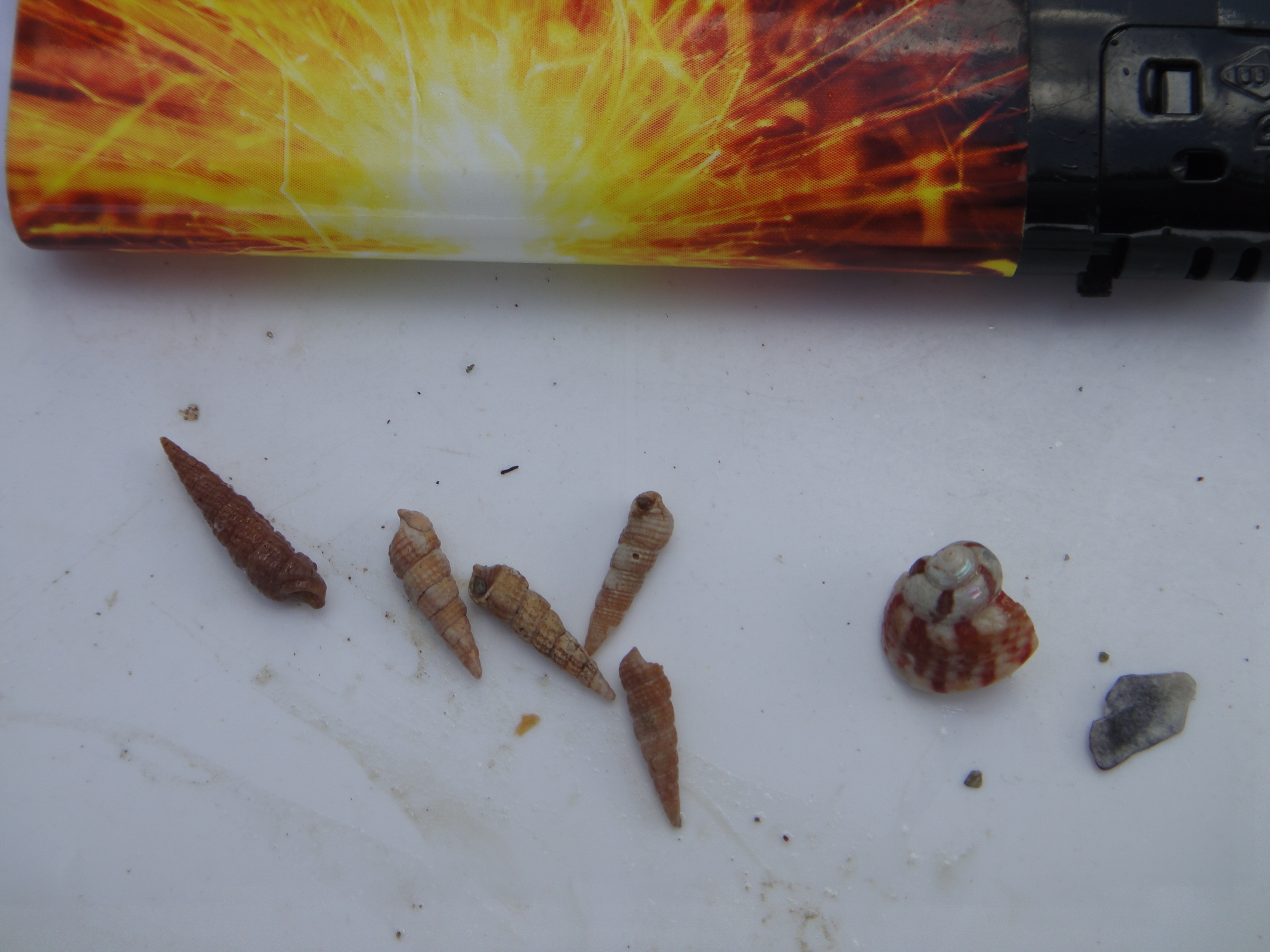
Figure 15: needle whelks (Bittium reticulatum) |
GRAB TWO: Latitude 50⁰08.549 Longitude 005⁰03.000 Eastings 182192.5234 Northings 31374.6040 Time in water (GMT) 16:30:40 DESCRIPTION: Grab sample was better sorted than grab one and dominated by finer gravel. Some live maerl was present, along with large and small shells and shell fragments. BIOTA: Flatworm, Serpulid Polychaetes e.g. Spirorbis spirorbis on rocks and larger shells, Keelworm (Pomatoceros lamarcki)
Click Images to Enlarge
Figure 16: bivalves and alive maerl from the grab
Figure 17: alive fragments of maerl from the grab sample |
FAILED GRABS – due to rock caught in grab, holding it open: 1. Latitude 50⁰08.598 Longitude 005⁰03.094 Eastings 182061.3980 Northings 31483.2658 Time in water (GMT) 16:22:16 Grab sample was poorly sorted, coarse gravel and rock with some shell fragments 2. Latitude 50⁰08.572 Longitude 005⁰03.056 Eastings 182117.1701 Northings 31429.4218 Time in water (GMT) 16:26:35 Grab sample was mostly gravel with some large rocks. Some shell and maerl fragments were spotted along with a top shell and an amphipod. |
|||||||||||||||||||||||||||||||
|
SIDE SCAN IMAGES
By analysing the side scan of the Falmouth Bay two features were
detected on the sea floor. One of the features (1) in Figure 18 can be identified as
a rock while the identity of the other feature (2) is to be discussed.
The idea of feature (2) being a scour mark is not reasonable due to the
fact it does not appear on the scan of the following return transect,
even though the areas should overlap in the scan prints. Another
suggestion is the feature could be a diver swimming in the same
direction as the sampling boat. The velocity of the sampling boat in
addition to the velocity of the diver would cause the potential diver to
appear longer on the side scan than in reality. The idea can be
supported with a made observation of a diver flag within that particular
region. Click Image to Enlarge
(1) (2) (3) (4) (5) Figure 18: This image shows 5 selected features from the recorded side scan.
|
|||||||||||||||||||||||||||||||||
|
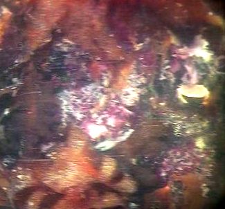
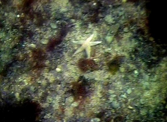
VIDEO SLED STILL IMAGES A video sled was used to gather real time footage of the surveyed area. The video started within the surveyed area closest to the shore and moved across the transects towards the sea-side. The footage showed a succession of finer sandy, calcareous sediment with small patches of seaweed and echinoderms to a more coarse calcareous sediment dominated with large kelp populations and crustaceans. When sediment is dumped in the spoil ground it smothers the life beneath it and may lead to patchy ecosystems and an ecological succession.
Figure 18: A snap shot from the video sled recording Figure 20: A snap shot from the end of the sled recording showing an edible crab (Cancer pagurus) on showing a common sea star (Asterias rubens). the right hand side. |
|||||||||||||||||||||||||||||||||
| Discussion | |||||||||||||||||||||||||||||||||
TRANSECT ANALYSIS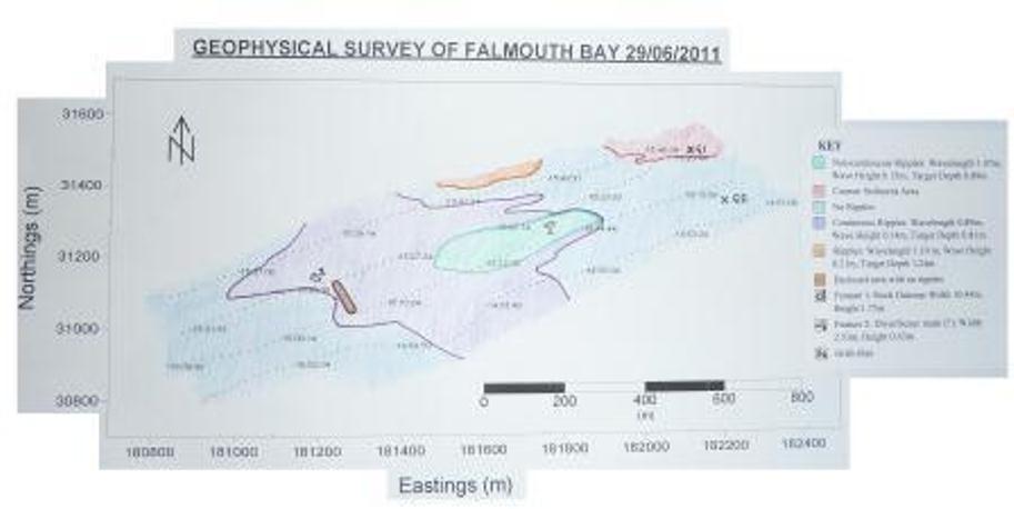 Upon analysis of the side scan imagery from the surveyed area, different areas were identified in terms of seabed roughness and bedform morphology. The blue area covering the largest proportion of the survey (31000N, 181000E) and (31200, 182200E) showed no indication of bedforms, with a uniform shade and no distinguishable shadows illustrating the presence of ripples or any other features. In the centre of the surveyed area, ripples were present in both a non continuous (wavelength 1.07m, wave height 0.15m and target depth 0.89m) and continuous form (wavelength 0.89m, wave height 0.14m and target depth 0.81m) (31200N, 181400E). The two types of ripples had very similar measurements, only to be distinguished between each other by the breaks in the banding within the non continuous area (green) to the east (31200N, 181700E). A further section of ripples is highlighted in orange (31400N, 181800E); characterised by the largest ripple morphology found in the survey area with a wavelength of 1.19m, wave height 0.21m and target depth of 1.24m. The final bedform section identified was in the north west of the survey (31400N, 182200E) (coloured red). This area shows a rougher sea bed with darker shading on the original imagery than the surrounding areas. Finally, two individual features were found within the survey area. The first (31200N, 181200E) clearly lifted above the seafloor with a measured height of 1.75m and covered an area 10.44m wide and had an irregular angular shape.
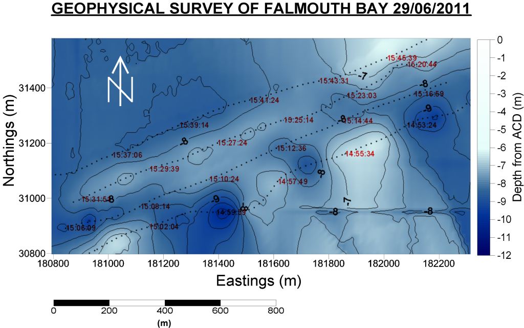
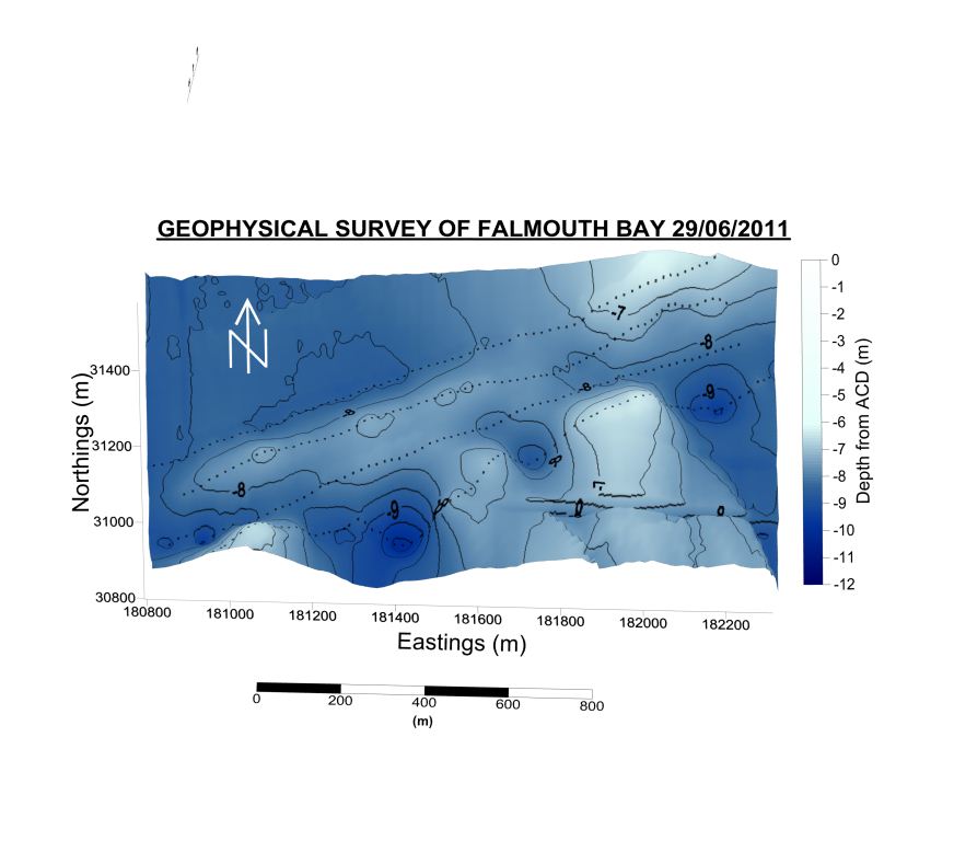
Figure 21: Geophysical survey map showing the
surveyed area
The second was much smaller and only appeared on one swath despite being at the outer boundary of the print out. The second feature (31200N, 181800E) had a straight rectangular shape area with a width of 2.53m and height 0.43m.
CONTOUR PLOT ANALYSIS
Figure 22: Survey contour map showing the depths of the surveyed area Figure 23: 3D map depicting the surveyed area Depth measurements were adjusted to give depth (m) relative to admiralty chart datum (ACD) *1. The preliminary adjustment was for the distance between the transducer and sea level height (draft height :1.14m )*2 , the secondary adjustment calculated the difference between the recorded water level height and ACD using interpolated corresponding tidal heights for each location. 4 transects were taken, each line being roughly 2km in length, aiming to be as parallel as possible. Transect 1 (31357N-182314E)- (30893N, 180845E) shows a 7m variation in depth (-5- -12m) with three -7m peaks and three noticeable troughs down to -12m troughs. Transect 2 (30893N- 180844E)- (31421N-182230E) shows a 2m variation in depth (-7- -9m) with three slight peaks (-7/-8m)and two troughs at -9m . Transect 3 (31493N -182197E)- (30986N-180872E) shows a 2m variation in depth (-7- -9m) with three -7m peaks and four -8m troughs. Transect 4 (31087N- 180793E)-( 31580N-182160E) shows a 2m variation in depth with one peak at -7m and one trough of -9m. When the four transects are combined and
interpolated using the surfer software package it can be seen that Falmouth bay has significant dune structures of up to 5m in height (-7m -
-12m), the gradient and quantity of dune structures decreases landwards, with the maximum difference on transect 4 (most landward) being only
2m with only 1 peak. This could be showing that the large dunes are attenuated closer to the surf zone, possibly by the increased interaction
and influence of tidal and wave energy observed in shallower waters. The sidescan data showed medium grey reflection from the seafloor; this
is normally an indication of medium sized sediment such as gravel/shells, and is grey due to slight adsorption of the acoustic pulse by loose
sediments . This observation was confirmed by the sediment samples collected using the van veer grabs. The grab samples were sieved, with the
majority of sediment being between 2-10mm in diameter. The grabs samples also contained a significant amount of biological artefacts, which
were not detected using the sidescan sonar. Following these observations; the deployment of an underwater video system enabled a visual survey
of the sampled area, confirming large amounts of kelp and, crabs and seastars. During the course of the geophysical survey, some minor errors occurred which prevented as much data
being collected in the allocated time. At the beginning of the survey the side scan printer did not function properly and so the first
transect was delayed. Due to the failure of the printer, the side scan was adjusted to a lower resolution to prevent conflicting software,
resulting in a lower contrast side scan and a more difficult interpretation of the bedforms. This problem also meant there was less time
overall throughout the day to carry out grabs at more than two different sites and so the ground truthing of certain areas became limited. |
|||||||||||||||||||||||||||||||||
| Conclusions | |||||||||||||||||||||||||||||||||
|
|
|||||||||||||||||||||||||||||||||
|
|
|
|
|
|
|
|
|
|
| Introduction | |||||||||||||||||||
|
The main aim of the estuary survey was to analyze the physical, chemical and biological characteristics of the Fal estuary. An estuarine system is a semi-enclosed coastal area with freshwater input in the form of rivers which dilutes the seawater and leads to a lower salinity. Terrestrial runoff into the estuary contains suspended particles of nutrient rich material. Tides and waves are also an important factor influencing the daily estuary conditions (Uncles, 2002). Eutrophication can be an issue due to the high nutrient amount in the river water. Half of the day was occupied by taking samples from the pontoon at 50° 12.970N, 005° 01.659W to document nutrient levels during tidal change. The later half of the day was on the Bill Conway recording transects and taking samples to document spatial change of nutrient levels. |
|||||||||||||||||||
| Methods | |||||||||||||||||||
|
Samples were taken on the pontoon from 09:00GMT to 11:26GMT. A horizontal Niskin bottle water sample was taken from the “riverside” of the pontoon on every hour, as well as at low water - 11:26GMT. When the Niskin bottle was brought to deck, a dissolved oxygen sample was immediately taken. Each 50ml water sample was filtered twice, with the two filter papers fixed in acetone to collect chlorophyll samples. The filtered water was used to collect a phosphate sample in a glass bottle, whereas silica was sampled in plastic bottle due to the nature of glass possibly interacting with the sample to be measured. Furthermore, for each filtered sample approximately five to ten milliliters were flushed through the glass fiber filter in order to clear it of any loose particulates that may contaminate the silica sample. Following this, 100 ml of unfiltered water was placed in a glass bottle containing Lugol's iodine to collect a preserved phytoplankton culture. In total four samples were taken at 09:00GMT, 10:00GMT, 11:00GMT, and 11:26GMT. However, at 11:00GMT oxygen and phytoplankton samples were not taken due to lack of sample bottles. In addition to the water collection, every half hour a YSI probe (6600 V2) was used on both the riverside and landside of the pontoon to record salinity, depth, pH, turbidity and temperature. Aboard Bill Conway, 9 transects in total were recorded with an Acoustic Doppler Current Profiler (ADCP). (Note: Transect 7** was not a full transect because the boat had to veer off course due to a ship blocking the course). The first four transects were carried out in between key stations of the river, whilst the latter five where carried out across the estuary at each key station. At the five stations a CTD was used to carry out a vertical profile of the water column. On the CTDs up-cast Niskin bottles were fired at three to four depths and from each of these, silica, phosphate, chlorophyll and dissolved oxygen samples were taken in the same way as on the pontoon. Additionally, at each station a secchi disk was used to gauge the light attenuation. Finally, 3 plankton net trawls were taken in total, 2 in the upper section of the river and the last at station 10 near the mouth. Each plankton net was thrown over the back of Conway for five minutes and a 500ml plankton sample taken and combined with formalin to fix the plankton sample.
Figure 24: Google Earth image showing the stations
and transects of the Estuary survey
|
|||||||||||||||||||
| Results | |||||||||||||||||||
|
PONTOON DATA Nutrients
ADCP SHIP TRACT DATA Transect 1 was the highest site upstream, recorded at the earliest time in the day; before the change in tide. This change in tide was at approximately 12:26. There was an ebb tide in the morning, showing similar velocity throughout the full water column. The sticks in the ship stick track show a fairly uniform, moderate flow in the southern direction (indicating the ebb) from the river to the mouth. There is, however, some variation in the stick directions in the west side of the channel. This could possibly be due to the fact that the water is shallower and apart from the main channel, increasing turbulence and resulting in more random flow directions. The average backscatter generally varies between 68-78dB, with some higher amounts in the top 2-3m as high as 107db. These high amounts of backscatter indicate increased levels of suspended plankton and material. For transect 2, velocity magnitude is fairly uniform throughout all depths, with a range of up to 0.282ms-1. The ship track shows a uniform southern flow with the ebb tide, which has decreased in the surface waters according to the approaching low tide at midday. The ship track on transect 3 shows a further decreasing surface flow, though it is still southern mean velocity. There are some much larger flows in the west of the estuary where the water is very shallow, within about 2m, which causes turbulence. Water velocity is also fairly uniform with depth. Backscatter is high in the surface waters, extending down to 6m, indicating high levels of suspended particulate and biological matter. Below this, there is very little variation. Transect 4 ship tracks show that the direction of flow has changed. It is now north, though surface velocity is very low. This shows the changing tide direction with the dominant flow pushing up into the estuary with the flooding tide. Both backscatter and water velocity are quite uniform with depth, showing little variation. Following the tidal pattern, the ship track for transects 5 and 6 show an increasing northerly flow in surface current. This is uniform in direction and with depth, though higher velocities are noted in shallower waters, up to 0.565ms-1, as opposed to 0.282ms-1 in lower waters. Backscatter is mostly constant with depth, though there are some areas in shallower waters showing small areas with significantly higher values. Some sticks observed in transects 7 and 8 are pointing in the opposite directions to the other sticks, indicating return flow along the sides of the estuary. Aside from this, high flow velocities are seen in the centre of the channel for transect 7, while the higher velocities are in the left for transect 8. Again, though water column velocity varies laterally across the channel, both transects show a moderately uniform vertical change.
Transect 9 is at
the bottom of the estuary near the mouth. Results show a moderate
southern flow, in contrast to the northern flow in the past few
transects. This is indicative of a change in tidal flow, as high tide
has passed. There is now an ebb tide again, which coincides with the
tidal height data for the evening. Once again, velocity is relatively
constant with depth, with some lateral variation. However, the average
velocity is the highest recorded for all stations, with the possible
exception of transect 1. The data for this station is however not helped
by a lack of detail in the plots. Backscatter changes with distance
along the transect, being highest in the west, as high as 105ms-1,
then reaching 70ms-1 in the east.
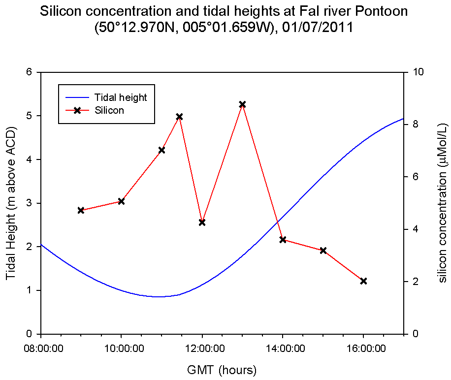
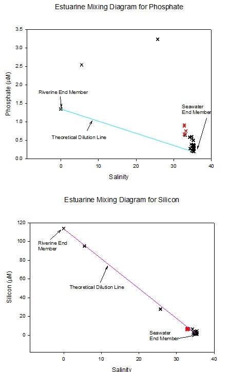
CHEMISTRY DATA In the Fal Estuary, the hydrological conditions (low riverine input) in conjunction with a macrotidal system produce a narrow range of high salinity values. All the samples taken were greater than 30 and ranged between 30.23 and 34.32. Consequently, all the data points which were sampled on the mixing diagrams are restricted to the higher salinity region and this ultimately creates issues when interpreting the behaviour of the chemical constituents within the estuary. Nevertheless, when the data was plotted with the riverine end members and with the addition of a theoretical dilution line (TDL- linking the two data points with the highest and lowest salinities), phosphate and silicate exhibited contrasting behaviour. PHOSPHATE- The phosphate estuarine mixing diagram illustrates a relatively low range of phosphate concentrations at high salinity values. The diagram highlights extreme non-conservative behaviour, indicating a possible input of phosphate to the estuary, possibly of anthropogenic origin and agriculture runoff. SILICON- The silicon concentration shows a linear relationship with respect to the salinity; an increase in salinity causes a decrease in silicon. The riverine end member has a salinity of 0, has a silicon concentration of 113.3µmol/L, the highest value in the estuary. Conversely, the seawater end member, salinity 34.32, has a concentration of 1.3µmol/L. Silicon behaves conservatively along the estuary following the theoretical dilution line precisely, suggesting that the chemical is equally mixed throughout the Fal and is not involved in (bio)chemical reactions. N.B. The initial readings on the CTD at station 1 and 2 for salinity were incorrect. This was caused by overnight crystalisation of salt on the conductivity sensor resulting in inaccurate measurements. Consequently, the salinities for some bottles of silicon and phosphate were measured using the thermosalinograph (readings indicated by red marks on the mixing diagrams). Therefore, the salinity values do not correspond to the macronutrient values sampled at depths below the surface
Oxygen
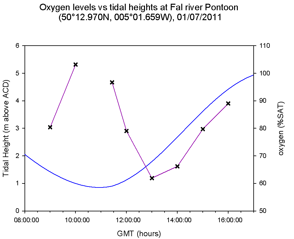
Surface oxygen saturation increased
dramatically from the head of the estuary (station 1- 92.9%) to the
mouth (station 10-99.4%). These surface concentrations must be in
equilibrium with the atmosphere, increasing down the estuary due to an
increase in oxygen exchange rate across the sea-surface interface due to
greater tidal and wave action and thus surface turbulence. The fact that
Station 1, at the head of the estuary has severely undersaturated oxygen
surface waters suggests a possible influx of deoxygenated water and/or
sewage waste, with a high BOD. All stations experienced an initial
increase within the first 10m. This is attributable to photosynthetic
activity where the photosynthetically active radiation is available and
mass oxygen is being produced. The mid estuary (station 5) exhibits the
highest oxygen saturation (>102%) at 5m depth indicating the area of
most primary production. Station 5 and 10 then continue to decrease with
depth which may be a result of zooplankton respiration and decomposition
and lack of available light for photosynthesis. However, at station 5
around 10 metres depth, the oxygen concentration begins to increase
again. This area of rapid decrease of oxygen saturation (5-10m depth)
coincides with a large increase in phosphate (0.6 µmol/L). This is an
indication of pollution causing an elevation of phytoplankton activity ,
an increase of organic material that has a high biological oxygen demand
and consequently a reduction in oxygen concentration. PLANKTON DATA The dominant taxa recorded include copepods (>25%) and copepod nauplii with a relatively high proportion of gastropod larvae (Figure 31).
LIGHT ATTENUATION
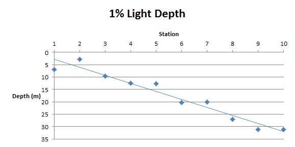
The 1% light depth graph (Figure 32 ) illustrates an increase with an
increase down the estuary. Station
1 showed rapid attenuation of light, which may be due to riverine input
and wind stress resulting in mixing, thereby increasing turbidity of the
surface layer.
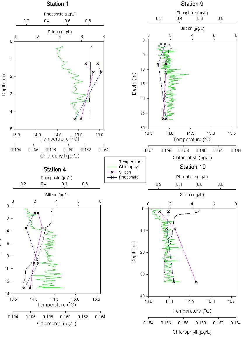
VERTICAL PROFILES Figure 33 is a vertical profile of stations 1, 4, 9 and 10, illustrating the relationship between silicon, phosphate, temperature and chlorophyll concentration. Temperature remains uniform with depth changing by 0.2 oC within a 4.4 metre change in depth. Naturally, silicon has a higher concentration than phosphate. However, at the surface they follow a similar trend, increasing from 6.3 and 0.9 to 6.9 and 0.91 respectively. The nutrients then appear to decrease in concentration which coincides with a peak in chlorophyll at 3.6 m.
Further down the estuary at station 4, there is a greater temperature gradient ( from 14.3 oC at the surface to 13.6 oC at 13m). At the surface both nutrients behave oppositely, with phosphate decreasing with depth and silicon increasing with depth. This trend continues down to 4m depth where the trend reverses, i.e. phosphate increases with depth and silicon decreases with depth. This coincides with a sharp increase in chlorophyll from 0.156 to 0.1583µg/L which, from this point, is relatively constant with depth.
Station 9 and station 10 represent the transition between the Estuarine environment and the marine environment. Significantly, chlorophyll and phosphate exhibit the same trends at each station; phosphate decreases from the surface to ~10m depth and increases at depths below 10m. Chlorophyll increases gradually with an increase in depth and is fairly homogenous below 10m. Importantly, there was a noticeable thermocline at station 10 that did not exist at the previous station. This is the onset of water column stratification indicating the beginning of the offshore structure. Silicon on the other hand increases with depth, which is associated with a large decrease in salinity (35.52 to 34.5 salinity), supporting the conservative behaviour shown in fig the estuarine mixing diagram for silicon. |
Click Images to Enlarge
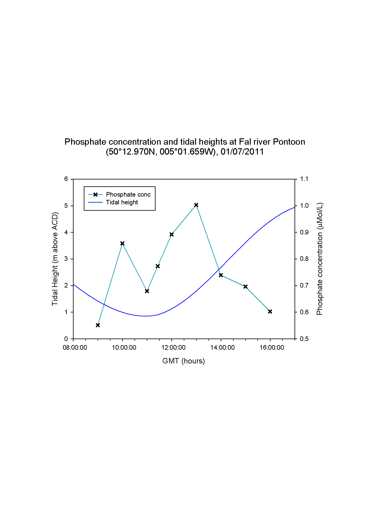
Figure 25: Phosphate concentration (light blue) and tidal height (dark blue) at Fal River Pontoon on July 1, 2011.
Figure 26 : Silicon Concentration (red) and tidal height (blue) at the Fal River Pontoon on July 1, 2011
Figure 27: Dissolved Oxygen (purple) and tidal height (blue) at the Fal River Pontoon on July 1, 2011
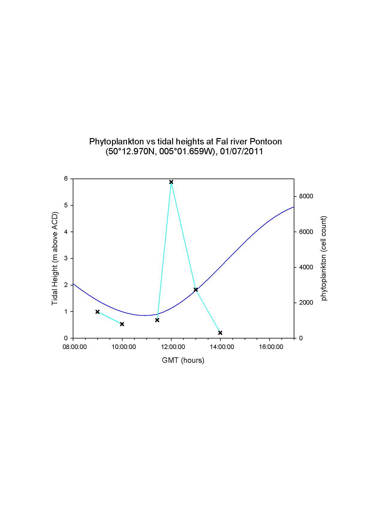
Figure 28: Phytoplankton (light blue) and tidal height (dark blue) at the Fal River Pontoon on July 1, 2011
Figure 29: Ship track images of Transects 1, 4, 7, and 9.
Figure 30: Estuary Mixing Diagrams for Phosphorus and Silicon
Figure 31: Breakdown of zooplankton cell count from the estuary trawl
Figure 32: 1% Light attenuation depth from Secchi Disk data
Figure 33: Vertical Depth Profiles for Stations 1, 4, 9 and 10 measuring Temperature, Chlorophyll, Silicon, and Phosphorus |
||||||||||||||||||
| Discussion | |||||||||||||||||||
| The observed
increase in nutrient concentrations following low tide may be explained
by the presence of a mussel farm a few hundred metres downstream from
the pontoon. As the tide begins to rise after 11:26 seawater would begin
to flow up the estuary taking with it the high artificial nutrient
concentrations maintained in the water of the mussel farm. This high
nutrient concentration allows growth of phytoplankton which is shown in
the phytoplankton cell counts and the chlorophyll concentration. The
decrease in oxygen at 12:00 can then be explained by this phytoplankton
increase and the increase in planktivorous heterotrophs which probably
occurs, all of which will use oxygen in respiration. The decrease in
nutrients at 14:00 shows nutrient consumption by phytoplankton. The
increase in silicon and phosphate at 11:26 and 10:11 cannot be explained
by the presence of the mussel farm and is unexpected in the data. It may
be because of variability in the concentration in the river flow but
this is unlikely. The change in salinity values over the tidal cycle show the salinity decreasing around low tide as the saline oceanic water moves out of the estuary. The salinities then increase again at 14:00 as seawater moves back into the estuary with the rising tide. The changes in temperature can also be explained by input of seawater into the estuary. Colder seawater moves into the estuary at 14:00, reducing the average temperature of the water column significantly. Earlier in the day at 10:00 the seawater moves out of the estuary to be replaced with warmer riverine water, increasing the average temperature. The decrease in chlorophyll concentration from the head to the mouth of the estuary can be accounted for by the assumption that zooplankton populations increase down the estuary resulting in an increase in grazing pressure upon the phytoplankton and microbial component of the estuary (Miller, 2004). (The data does not support the assumption that there is an increase in zooplankton down the estuary, but the methods for zooplankton data collection are too subjective to be reliable). However, the fact that there is an overall decrease in silicon and phosphate concentrations down the estuary allowing phytoplankton to exist in the upper estuary (uptake of nutrients in the upper estuary by primary producers) underpins the inverse zooplankton-phytoplankton relationship down the Fal estuary.
There is an apparent
relationship between silicon concentration and salinity which cannot be
accounted for by physical mixing processes shown in the mixing diagram.
This suggests some component of biological uptake of silica by
pelagic/benthic phytoplankton (i.e. diatoms). This suggests that the
silicon is behaving as a pseudo-conservative element, but this is
difficult to say without the flow rates of the estuary. |
|||||||||||||||||||
| Conclusion | |||||||||||||||||||
|
The changes in phytoplankton cell counts and chlorophyll correlate well and can be explained by artificially high concentrations of nutrients moving up the estuary from the mussel farm with the rising tide. The lower oxygen saturation following this is believed to be directly caused by higher amount of phytoplankton and zooplankton these are presumed to support consuming oxygen in respiration. The salinity and temperature time series show the expected variation with time as colder, more saline seawater moves in and out of the estuary with the tide. The Fal estuary can certainly be categorised as a well mixed, tidally dominated estuary. The physical profiles (temperature and salinity) are relatively uniform throughout. The upper part of the estuary represents the region of most uniform physical conditions due to the low riverine freshwater input coupled with the relatively strong wind stress. Progression down the estuary shows a very gradual stratification in the water column but only becomes apparent at station 10, when the offshore environment becomes prominent. |
|||||||||||||||||||
|
|
|
|
|
|
|
|
|
|
|
During the three surveys within one week on the Fal estuary, the Falmouth Bay and offshore region the biological, chemical and physical conditions have been measured and analysed. The weather during the sampling period was dominated by a mix of clouds and sun with a little rain on the first day. The offshore region showed a characteristic frontal system with a mixed region on the estuary side and stratification on the offshore side. However, due to a long cold weather period in June the stratification is relatively weakly developed. The coastal front was localised near 50° 06.07N, 5° 00.02 W. The Fal estuary is influenced by the strong daily tides, whereas the freshwater input barely influences the estuary conditions. Differences from last years’ findings occur in the silicon concentration which is highly conservative, in contrast to the removal of silicon last year. A phosphate input by anthropogenic activities (for example the mussel farm and agriculture) causes eutrophication of the estuary. For both the estuarine and offshore system, it is important to consider the interactions between all physical, chemical and biological factors. During the geophysical analysis a lack of distinct bedforms on the seabed and a homogeneous sediment type was discovered, although when studied in detail differing sizes and types of ripples were found. As the video transect moved away from the spoiling ground of the survey area succession could be seen with the biota becoming more diverse. |
|
|
|
|
|
|
|
|
|
|
|
Bird, E. (1998) The Coasts of Cornwall. Alexander Associates, Fowey, Cornwall, 237 pp.
Beardall, J., Foster, P., Voltolina, D. & Savidge, G. (1982)
Observations on the surface water Blondel, P., 2009. 'The Handbook of sidescan sonar', 316pp. Berlin, Springer Bowen, G. G., Dussek, C. and Hamilton, R. M., 1998, ‘Pollution resulting from the abandonment and subsequent flooding of Wheal Jane Mine in Cornwall, UK’, Geological Society, London, Special Publications, 128, 93-99 F.D. Marine Ltd. No Date. ‘Multipurpose Vessel: Grey Bear Shallow Draft Work Boat’, 1-2. Fogg, G.E., Egon, B., Hoy, S., Lochte, K., Scrope-Howe, S. and Turley, C.K.M., 1985. Biological studies in the vicinity of a shallow-sea tidal mixing front. 1.Physical and Chemical Background. Philosophical Transactions of the Royal Society of London B, 310, 407-433
Gubbay, S., Baker, M., Bett, B. and Konnecker, G., 2002. The Offshore
Directory: Review of a selection of habitats, communities and species of
the north-east Atlantic, WWF North-east Atlantic Programme, 49-54. Head, P.C., (1985), “Practical Estuarine Chemistry: A Handbook”, Cambridge University Press, 337pp. Langston, W.J., Chesman, D.S., Burt, G.
R., Hawkins, S.J., Readman, J., and Worsfold, P., 2003. 'The
Characterisation of European Marine Sites. The Fal and Helford', JMBA,
vol 8. Miller, C.B., (2008), “Biological Oceanography”, Blackwell publishing, Chapter 1 “The spring Phytoplankton bloom”, 1-20 pp. Mullin, J. B., and Riley, J. P., 1955. The colorimetric determination
of silicate with special reference to sea and natural waters, Analytica
Chimica Acta, 12, 162-176. Parsons T. R. Maita Y. and Lalli C. (1984) “ A manual of chemical and
biological methods for seawater analysis” 173 p. Pergamon. Pirrie, D., Power, M. R., Rollinson, G., Hughes, S. H., Camm. G. S. and Watkins, D. C., (no date) ‘Mapping and visualisation of historical mining contamination in the Fal Estuary. Cornwall’, [online] Cambourne School of Mines, University of Exeter, Available at: <http://www.btinternet.com/~mattpower/Fal/home.htm> [Accessed 4/7/2011] Pirrie, D., Power, M. R., Rollinson, G., Camm, G. S., Hughes, S. H., Butcher, A. E. and Hughes, P., (2003) “The spatial distrubution and source of arsenic, copper, tin and zinc within the surface sediments of the Fal Estuary, Cornwall, UK”, Sedimentology, 50(3), 579-595
Sharples J.,
Simpson J. H. (2009) Shelf Sea and Shelf Slope Fronts. Elsevier
Ltd.weatheronline.co.uk (accessed: 5 July 2011)
Stapleton, C. and Pethick, J. (1996) The Fal Estuary: Coastal
Processes and Conservation. Report by the Institute of Estuarine and
Coastal Studies. University of Hull for English Nature. Reference list for Equipment Images: Transmissometer: Sensor Information, Chelsea Technologies Group Limited, [Online], Available: http://www.chelsea.co.uk/ajoomla15/products/sensors, Accessed 2011,July 5th ADCP: Equipment Images, Craney Island Eastward Expansion Project Infomation, [Online], Available: http://web.vims.edu/physical/projects/craney/adcp.gif, Accessed 2011, July 5th Side Scan:http:Side Scan Sonar, [Online], Available: //www.absoluteastronomy.com/discussionpost/Looking_for_a_Side_Scan_Sonar_product_Best_3D_sonar_to_connect_to_Furuno_NavNet_3D_Looking_to_buy_in_the_2_to_3K_price_range_any_suggestions__T_96480609, Accessed 2011, July 5th Vertical Plankton Net: Plankton Nets, [Online], Available: http://el.erdc.usace.army.mil/zebra/zmis/zmishelp/plankton_nets.htm, Accessed 2001, July 5th TS Probe: Image of Temperature Salinity Meter, U-Therm International (h.k) Limited, [Online], Available http://labkits.en.made-in-china.com/product/deqJIfKkkbWy/China-Conductivity-TDS-Salinity-Temperature-DO-PH-Meter.html, Accessed 2011, July 5th Fluorometer: Sensor Package Details, River, Estuary and Coastal Observing Network, [Online}, Available http://recon.sccf.org/about/sensor_details.shtml, Accessed 2011, July 5th Spectrophotometer, [Online], 2011. Available: http://www.britannica.com/EBchecked/topic/558879/spectrophotometer [accessed 2011, July 5th].
|
| Disclaimer: The views and opinions expressed on this website are those of the students named at the beginning of the website and do not reflect those of the University of Southampton or the National Oceanographic Centre. |


.JPG)